
In the previous article Part 1 - What is ML?, you got an introduction to machine learning, and you saw how it works from a programmer's perspective by having you create answers and data, and letting a computer infer the rules that determine them.
This is fundamentally different from traditional programming, where you have to figure out the rules, express them in code, and then have them act on data to give answers.
You created your first neural network, a single layer with a single neuron, to figure out the relationship between two numbers.
In this part, we'll start by looking at computer vision and how a computer can learn to see. We'll start simple, and we'll build from there.
So in understanding vision, ultimately it's all seeing and recognizing things in a field of view. So for example, consider the items of clothing.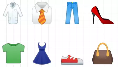 If I were to ask you which ones were shoes, you'd probably know right away that it's the high heel and the sneaker. But how did you know that? How could you teach someone who has never seen a shoe before what a shoe is so that they could then tell the difference? What are the rules that make a shoe a shoe?
Looking back at the data, how would you come up with the rules to determine a shoe? If it's red, it's a shoe, maybe. Well, that works for this data, but we all know that that won't work for all shoes.
Computer vision is the field of taking pixels and recognizing what's in them. And the same kind of pattern matching we've been discussing can be used here. But in order to train a neural network to recognize the contents of images, we need data, and we need labeled images.
Fortunately, there's an easily available data set called Fashion MNIST. This has 70,000 images sorted and labeled in 10 categories. The images are small. They're 28 by 28. But despite this, they're still recognizable. You can tell that this image is a boot.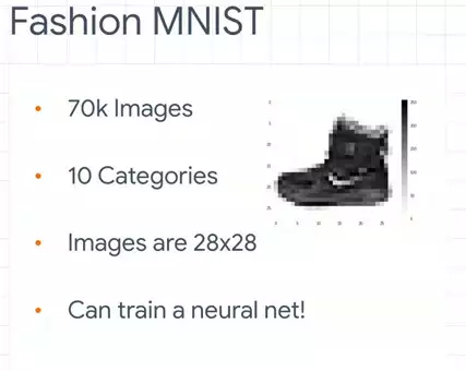 And because they're small, we can train a neural network quickly using them.
We'll start by loading the data.
import tensorflow as tf

mnist = tf.keras.datasets.fashion_mnist
(training_images, training_labels), (test_images, test_labels) = mnist.load_data()
In Keras, there's some built-in data sets that can be loaded with a single line of code. Python can return multiple values from a single call, and four values are returned here. First is a set of training_images and training_labels, and then is a set of test_images and test_labels.
You might wonder why our images have been split into two sets. There's one for testing and this one for training. The idea here is really simple. We'll take a subset of our images -- in this case, 60,000 of the 70,000 -- that we'll train the neural network with. We'll then use the other 10,000 to see how well it performs on images it has never seen before.
Think about how you would teach someone who has never seen a shoe before what a shoe looks like. You'd probably get a bunch of shoes and show them. But then there's no point in testing that person on the shoes that you've just shown them, because in that case, you've already told them that those are shoes. Instead, you'll get a bunch of stuff that they haven't seen before, and have them pick out which ones are shoes. It's the same principle here, and it's one that you'll commonly see in building neural networks with machine learning.
So, back to our data -- we have four lists, one for training images, one for training labels, one for test images, and one for test labels. Our images of the 28x28 pixel arrays for the clothing items like the boot. And the labels are numbers from 0 to 9, indicating the appropriate item of clothing.
Think about this for a second. Why do you think that it would be a number, such as 9, and not a piece of text, like boot? Well, there's two main answers to this. The first is that computers deal better with numbers, and we train our neural nets using numbers. The second, a little more subtle, but very important, is that, by using a string here that said boot, we'd be introducing a bias that the neural network will need to understand the English word for the clothing item. But we don't want that bias. So we use the number 9 instead of the text for ankle boot, which I can then present here in a few different languages.
So here's what our neural network definition will look like.
model = tf.keras.models.Sequential([tf.keras.layers.Flatten(),
                                    tf.keras.layers.Dense(128, activation=tf.nn.relu),
                                    tf.keras.layers.Dense(10, activation=tf.nn.softmax)])
In the Part 1, you saw a neural network with a single layer containing a single neuron. Now we have one with three layers. The first layer is called a Flatten, and this is a special type of layer in Keras. There's no neurons here. But the idea of the function is to take the rectangular shape of the data, the 28 by 28, and flatten that into a one-dimensional array that can be processed by the next layer. Hence the name, flatten.
This is followed by a Dense layer. Now, note that there are 128 neurons in this layer. It's significantly larger than the one-neuron single layer that we used last time. This is followed in turn by another dense layer, this time one with 10 neurons in it.
There's a few important details here that you need to consider and need to remember when designing neural networks. To understand what the network is for, it's always good to look at the top layer and the bottom layer for their shaping. In this case, the top layer takes 28x28 for its input, which is the size of the images in our data set. Remember that, when building neural networks, all data being fed into training has to be the same size. In this case, it's easy because the data was already in 28x28 for us. But later, you'll see that you often need to pre-process your data to get it ready for training.
On the output side, we have 10 neurons. Remember, that there were 10 different types of clothing in the data set. This is not a coincidence. The job of each of these neurons will be to calculate the probability that a piece of clothing is for that particular class.
You're probably also wondering what activation parameter are. Well, they're another place where neural networks do a lot of math. But fortunately, most of it is encapsulated in parameters for you by TensorFlow. Layers in TensorFlow can have an activation function run on them. This is code that executes while the network is learning. They can be really useful, and can save you a lot of time writing code for yourself.
The relu function here is pretty simple. It basically says that if the output of a neuron is less than 0, set it to 0. The reason for this is that negative outputs could skew results downstream, canceling out positive outputs elsewhere. So we'll just throw them away.
Softmax, commonly seen on the final layer if there are multiple categories, simply helps you find the most likely candidate. Remember earlier that I said that each of the neurons in the bottom layer will be a probability that the item of clothing matches that class. That could give you something like this. And instead of you writing code to look through each value and find the largest, softmax will set the largest to 1 and the rest to 0. So now, to get the correct class, you just need to find the 1.
To illustrate the learning a bit, think about all of the pixel values, which are numbers from 0 to 255, being fed into a neuron called n0. 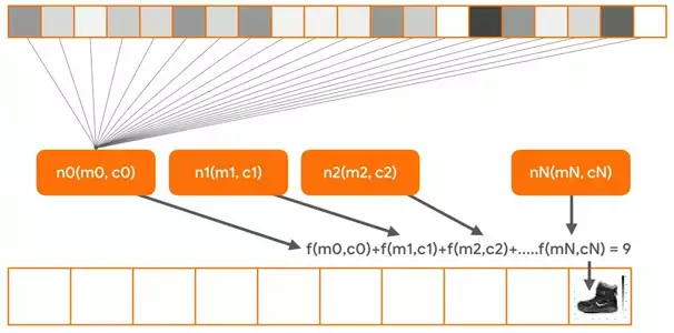 And its parameters, n0 and c0, are guessed. The same happens for every neuron in the network. Each neuron is initialized with random parameters, m and c. And when the pixels of each image in the training set -- and that's all 60,000 of them -- are fed in one by one, when all the totals from all the neurons are added up, we'll get an answer. The loss function then calculates how good or how bad that answer is, and the optimizer then tweaks the m's and the c's of the neurons to give it another try.
Over time, the values within the neurons will change so that the answers for the training data are fit as accurately as possible to the labels in the training data. This is the same learning that we saw in the single-neuron example in the last part.
So on the loss function and optimizer, we specify them when we compile the model.
model.compile(optimizer = tf.keras.optimizers.Adam(),
              loss = 'sparse_categorical_crossentropy',
              metrics=['accuracy'])
This time we'll use an optimizer called adam, which is a particularly good one for a task like this, and a loss function called sparse_categorical_crossentropy. Note that when you're classifying multiple categories -- and we have 10 here -- you're going to need something categorical.
Don't worry if you don't understand what this is what the options are yet. Just go with it. And over time, you'll learn good optimizers and loss functions for specific scenarios.
Next up, we just want to fit the training data to its labels.
model.fit(training_images, training_labels, epochs=5)
And we'll run it for just five epochs this time, because there's a lot of data there. Last time when we did the y equals 2x - 1, we then used model.predict to test our network. That worked for a single value. You can also use model.evaluate to pass it in to a list of test data. It takes the test images, gets its prediction, compares that to the answer in the test labels, and then calculates how many it got right and how many it got wrong, returning you an answer. It's a nice one line of code to help you test.
test_loss, test_acc = model.evaluate(test_images, test_labels)
And if you want to see the predictions for yourself, you can of course do a model.predict.
classifications = model.predict(test_images)
If you pass it in multiple images, it will return a list of all of the predictions for the respective images.
So that's a run through your first computer vision neural network.

No comments yet