
Previous Part 5: Classifying real-world images
In this part where we'll take what you've learned about convolutional neural networks in the previous few parts and apply them to a computer vision scenario that was a Kaggle challenge not that long ago.
The dogs versus cats data set has 25,000 images of cats and dogs in various poses. It was used for a Kaggle challenge a few years ago in determining state-of-the-art computer vision techniques. In the next few minutes, you'll see how to use what you've learned so far to build a classifier for cats and dogs that's over 96% accurate on the training site.
As before, you're going to split the data into training and validation directories. And each of these will have cats and dogs sub-directories. You will then be able to train a classifier on cats and dogs images using a generator that pulls from the training sub-directories and which validates by using a generator that pulls from the validation sub-directories.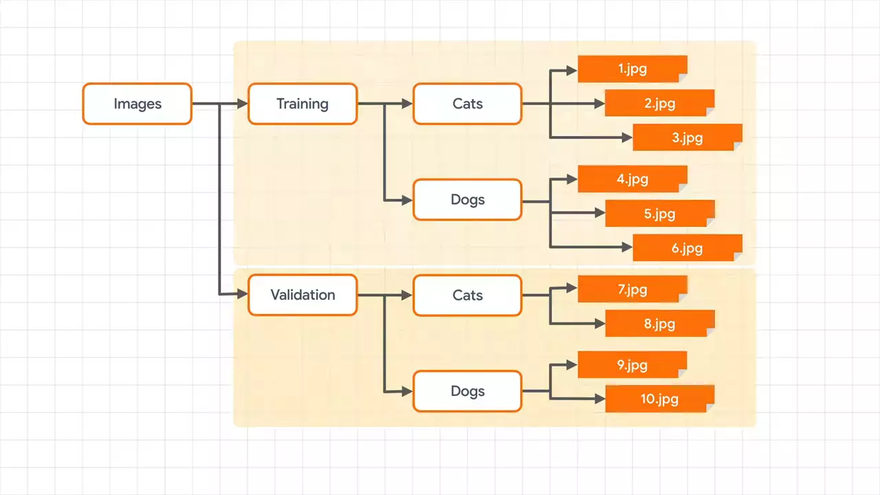 So to get started, let's first import an image data generator, which allows us to use them.
from tensorflow.keras.preprocessing.image import ImageDataGenerator
For our training data, we'll then simply create an image data generator and flow from the training directory.
TRAINING_DIR = "/tmp/cats-v-dogs/training/"
train_datagen = ImageDataGenerator(rescale=1.0/255.)
train_generator = train_datagen.flow_from_directory(TRAINING_DIR,
                                                    batch_size=250,
                                                    class_mode='binary',
                                                    target_size=(150, 150))
Note that the image data generator will handle normalizing the images by dividing their byte values by 255 to turn a value from 0 to 255 into a value from 0 to 1.
To get the training images from the training sub-directories, we can call flow_from_directory, passing in a bunch of parameters -- the first of which, of course, is the training directory itself. This should only contain sub-directories for which we'll provide the labels for the classes. We have cats and dogs sub-directories. So we'll have cats and dogs labels.
Next is our target_size. And as the images come in many sizes, we'll need to have a consistent shape to feed into the neural network. I've set them to be 150x150 here. But you can choose whatever you want, of course.
All images, regardless of their shape, will end up as 150x150. So choose carefully. And remember when creating your model to have the input layers use the same dimensions.
Next, choose a batch_size for which the images will be loaded. Pick something that divides evenly into a step size that you'll use later. So for example, if I have 22,500 training images, and that's taking 90% of the data for training, and then a batch size of 250, then I will need 90 steps to load this into the neural network.
Finally, there's the class_mode. And as the two classes, we'll set it to binary.
For validation you'll do exactly the same. Except, of course, that you want to flow from the validation directory and not the training one.
VALIDATION_DIR = "/tmp/cats-v-dogs/testing/"
validation_datagen = ImageDataGenerator(rescale=1.0/255.)
validation_generator = validation_datagen.flow_from_directory(VALIDATION_DIR,
                                                              batch_size=250,
                                                              class_mode='binary',
                                                              target_size=(150, 150))
And here's where you define your model.
model = tf.keras.models.Sequential([
    tf.keras.layers.Conv2D(16, (3, 3), activation='relu', input_shape=(150, 150, 3)),
    tf.keras.layers.MaxPooling2D(2, 2),
    tf.keras.layers.Conv2D(32, (3, 3), activation='relu'),
    tf.keras.layers.MaxPooling2D(2, 2),
    tf.keras.layers.Conv2D(64, (3, 3), activation='relu'),
    tf.keras.layers.MaxPooling2D(2, 2),
    tf.keras.layers.Flatten(),
    tf.keras.layers.Dense(512, activation='relu'),
    tf.keras.layers.Dense(1, activation='sigmoid')
])
This should look familiar by now. It is a convolutional neural network. I've designed this one with three convolutional layers, each paired with a max pool layer.
The first convolutional layer will learn 16 filters, the next 32, and the next 64. It's important to remember the input shape. Remember earlier we resized everything to be 150x150. And that's what we use here. The 3 is for the color channels. If you use a different size, make sure to adjust this to match. And similar for your output layer. This should match to the number of classes in your model. One exception, which we're following here, is that a binary classifier can get by with just one neuron, provided you use a sigmoid activation function, which sets it to 0 for one class and 1 for the other.
If we take a look at our model summary, it looks like this.
Layer (type)                 Output Shape              Param #
=================================================================
conv2d_21 (Conv2D)           (None, 148, 148, 16)      448
_________________________________________________________________
max_pooling2d_21 (MaxPooling (None, 74, 74, 16)        0
_________________________________________________________________
conv2d_22 (Conv2D)           (None, 72, 72, 32)        4640
_________________________________________________________________
max_pooling2d_22 (MaxPooling (None, 36, 36, 32)        0
_________________________________________________________________
conv2d_23 (Conv2D)           (None, 34, 34, 64)        18496
_________________________________________________________________
max_pooling2d_23 (MaxPooling (None, 17, 17, 64)        0
_________________________________________________________________
flatten_7 (Flatten)          (None, 18496)             0
_________________________________________________________________
dense_14 (Dense)             (None, 512)               9470464
_________________________________________________________________
dense_15 (Dense)             (None, 1)                 513
=================================================================
Total params: 9,494,561
Trainable params: 9,494,561
Non-trainable params: 0
You can see the familiar resizing of the image as it travels through the network by convolutions and pooling. By the end, you can see that we have 9 and 1/2 million trainable parameters. So this can take a while.
I've chosen to use RMS prop as the optimizer here.
from tensorflow.keras.optimizers import RMSprop
model.compile(optimizer=RMSprop(lr=0.001), loss='binary_crossentropy', metrics=['acc'])
It's set with a high learning rate. And you can tweak this to try for better performance on your network.
Finally, we'll train the network by specifying the training and validation generators as our data sources.
history = model.fit(train_generator, epochs=15, steps_per_epoch=90,
                    validation_data=validation_generator, validation_steps=10)
Don't forget to set the steps per epoch and validation steps for performance. And these should be calculated by dividing the amount of data by the batch size. This gives us 90 and 10, respectively in this case.
That gives you everything you need to train a cat versus dogs classifier.
Next Part 7 - Image augmentation and overfitting

No comments yet