
In the previous part 2 - First steps in computer vision, you built a neural network that could recognize items of clothing.
Now that you've looked at fashion example for computer vision, you've probably noticed a big limitation for computer vision with these example. And that was that you could only have one item in the picture, and then it had to be centered, and it to be well-defined. So shoes had to face left, for example. A neural network type called a convolutional neural network can help here. It'll take us a little time to build up to it. And in this part, we'll talk all about what convolutions are and how they can be used in combination with something called pooling to help a computer understand the contents of an image.
It's going to take a little while to put it all together. But let's start with just understanding what a convolution is before you can start using one. The idea behind the convolution is very similar to image processing with filters. If you use something like Photoshop before, it has filters to do things like sharpening an image or adding motion blur. So while the effect is complex, the process behind it is quite simple. So let's take a look at it in action.
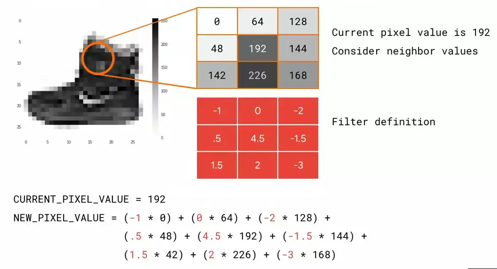 On the left, I have an image of a boot from the fashion MNIST dataset. On the right, I have a representation of nine of the pixels in the image. I'm going to call the center one my current pixel, and all of the others are its neighbors. I define a filter, which is a set of values in the same shape as my pixel and its neighbors. So for example, if I had one neighbor in each direction for a 3x3 grid of pixels, I'd have a 3x3 grid in my filter, too. Each value in the filter can be called a weight. So to calculate a new value for my pixel, all I have to do is multiply each neighbor by their weight, my current pixel by its weight, and then add them all up. And I'm going to do this process for every pixel in the image. The result will be a transformed image.
So for example, if you look at the picture on the left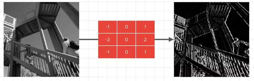 if I apply the filter in the middle to it, I'll get the picture on the right. This filter has led to a huge emphasis on vertical lines. They really pop now. And similarly, this filter leads to an emphasis on horizontal lines.
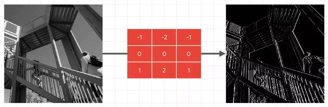 So you might be wondering at this point, what does this have to do with computer vision? Ultimately, the goal of trying to understand what an item is isn't just matching the raw pixels to labels like we did with the fashion example. But what if we could extract features from the image instead, and then when an image had this set of features, it was this class, or if it had that set of features it was that class? And that's the heart of what convolutional neural networks do. They process the images down into raw features, and then they find sets of features that will match the label. And they do this using filters. And just like neurons learned weights and biases to add up to what we needed, convolutions will learn the appropriate filters through an initial randomization, and then using the loss function and optimizer to tweak them for better results.
So for example, take a look at these images. 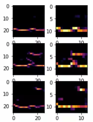 And you can see how they've been transformed by filters. And these filters learned how to isolate and abstract features within them. You can see, for example, that something like our horizontal line detector was able to detect a commonality in these images. And they're all shoes. And that line is the sole of the shoe.
But if you consider these images with the same filter, they had different results. 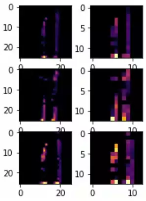 So if a lot of pixels are lighting up with the horizontal line filter, we could kind of sort of describe that as a sole detector.
You might hear that phrase a lot -- "detector." But what it's referring to is ultimately a filter that can extract a feature that can be used to determine a class. I first heard it in the cats versus dogs classifier, which we'll look later, when somebody visualized a floppy ear detector, which determined something was a dog and not a cat.
One other thing that you might have noticed in the previous picture was also that the resolution of the images was decreasing. This is achieved through something called a pooling. The idea here is pretty simple. If there is a way that we can extract the feature while removing extraneous information, we can actually learn much faster.
Now, let's take a look at how this works. The concept is actually quite simple. Imagine this is a chunk of our pixels.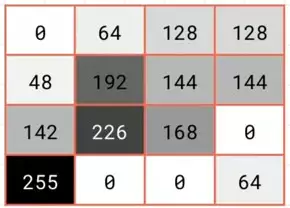 To keep it simple, I'm just going to have them as monochrome. We then look at them in blocks of 2x2, and then we'll only keep the biggest value
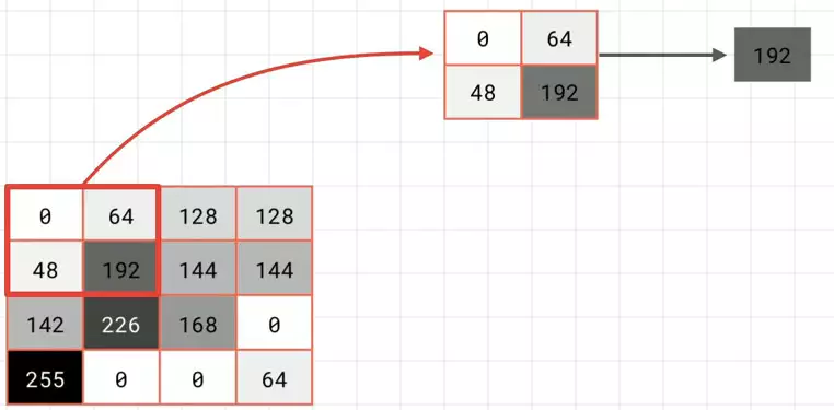 which in this case is 192. We then repeat the process for the next 2x2, and keep the biggest, which is 144; and the next, which yields 255; and the next, which yields 168.
 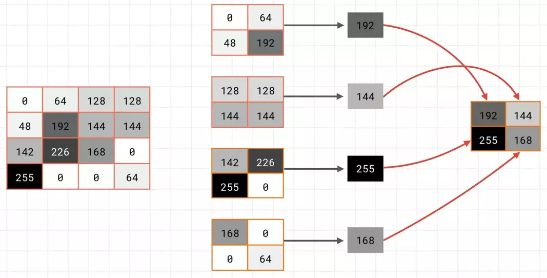 We then put these four results together to yield a new 2x2 block. And this contains what had been the largest values in the 2x2 constituents of the previous 4x4 block.
We've now reduced the size by 75%, and maybe -- just maybe -- we've kept the important information. So let's see what this actually looks like. Here is the image that we had filtered earlier to detect vertical lines. 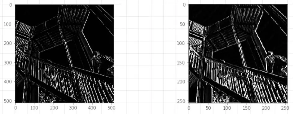 On the left is what it looks like before pooling. And on the right is what it looks like after pooling in the way that we just demonstrated.
Notice how the information hasn't just been maintained. You could argue that's also been emphasized. Pooling is an important way, also, of reducing the amount of information your model has to process. If you think about it, say you want to learn 100 filters. That means you would have to keep track of 101 versions of your image -- the original plus the results of what it would look like after the filters have been applied. If you have thousands of images, you'll soon start to eat memory. And that's just one layer. What if you had another layer beneath this that also learned 100 filters? That would mean each of your first 100 will also have 100 products from it, giving you 10,000 images for every image you need to train. Any technique that can reduce size while keeping this information is obviously very valuable.
So now that we've seen what a convolution is, and how it works, as well as how it can go hand-in-hand with pooling, let's take some time to see how to code for them.
So let's take a look at some convolutions in action. I want to talk about, for example, if you were going to classify a shoe instead of the one that you had in fashion MNIST. One of the ways of doing this is with convolutions. And in this part, you'll just take a quick experiment to see how the filters of convolutions work.
So we'll start by importing some of the required Python libraries.
import cv2
import numpy as np
from scipy import misc
i = misc.ascent()
And one of the things that's built into these libraries is this image called ascent. So we can use the pyplot library to draw it, so we can see what it looks like.
import matplotlib.pyplot as plt
plt.grid(False)
plt.gray()
plt.axis('off')
plt.imshow(i)
plt.show()
And it's a person walking up some stairs. 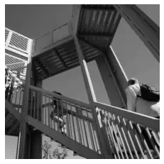 I'm now copy that into a
 numpy array so you can manipulate it.
i_transformed = np.copy(i)
size_x = i_transformed.shape[0]
size_y = i_transformed.shape[1]
And here I've defined a number of different filters.
# This filter detects edges nicely
# It creates a convolution that only passes through sharp edges and straight
# lines.

#Experiment with different values for fun effects.
#filter = [ [0, 1, 0], [1, -4, 1], [0, 1, 0]]

# A couple more filters to try for fun!
filter = [ [-1, -2, -1], [0, 0, 0], [1, 2, 1]]
#filter = [ [-1, 0, 1], [-2, 0, 2], [-1, 0, 1]]

# If all the digits in the filter don't add up to 0 or 1, you
# should probably do a weight to get it to do so
# so, for example, if your weights are 1,1,1 1,2,1 1,1,1
# They add up to 10, so you would set a weight of .1 if you want to normalize them
weight  = 1
Remember the 3x3 filters that we were showing? I'm just implementing them as three arrays of three items.
And one other thing that I've done is added a weight to this so that one of the things is that all the digits should add up to 1. But if they had to add up to something more than that, then you can multiply them out by a factor to normalize them. So for example, if they added up to 10, you could set the weight to 0.1 so the final result would be normalized back to 1.
for x in range(1,size_x-1):
  for y in range(1,size_y-1):
      convolution = 0.0
      convolution = convolution + (i[x - 1, y-1] * filter[0][0])
      convolution = convolution + (i[x, y-1] * filter[0][1])
      convolution = convolution + (i[x + 1, y-1] * filter[0][2])
      convolution = convolution + (i[x-1, y] * filter[1][0])
      convolution = convolution + (i[x, y] * filter[1][1])
      convolution = convolution + (i[x+1, y] * filter[1][2])
      convolution = convolution + (i[x-1, y+1] * filter[2][0])
      convolution = convolution + (i[x, y+1] * filter[2][1])
      convolution = convolution + (i[x+1, y+1] * filter[2][2])
      convolution = convolution * weight
      if(convolution255):
        convolution=255
      i_transformed[x, y] = convolution
Now here's is just simply a loop going over the image and multiplying out the relevant pixel and its neighbors by the relevant item in the filter. Once it's done that, we can plot it to see the result.
# Plot the image. Note the size of the axes -- they are 512 by 512
plt.gray()
plt.grid(False)
plt.imshow(i_transformed)
#plt.axis('off')
plt.show()
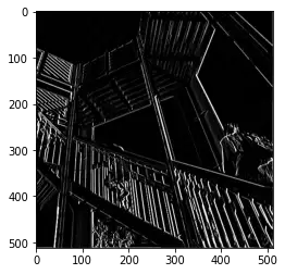 And you can see the filter is really emphasizing the image's vertical lines.
For example, if you change to a different filter like this one
filter = [ [-1, 0, 1], [-2, 0, 2], [-1, 0, 1]]
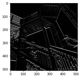
And we'll see the one that really emphasizes the horizontal lines.
So you can consider following filter values and look at what their impact on the images is, or you can experiment with your own.
So for example, this is implementation of a simple pooling.
new_x = int(size_x/2)
new_y = int(size_y/2)
newImage = np.zeros((new_x, new_y))
for x in range(0, size_x, 2):
  for y in range(0, size_y, 2):
    pixels = []
    pixels.append(i_transformed[x, y])
    pixels.append(i_transformed[x+1, y])
    pixels.append(i_transformed[x, y+1])
    pixels.append(i_transformed[x+1, y+1])
    pixels.sort(reverse=True)
    newImage[int(x/2),int(y/2)] = pixels[0]

# Plot the image. Note the size of the axes -- now 256 pixels instead of 512
plt.gray()
plt.grid(False)
plt.imshow(newImage)
#plt.axis('off')
plt.show()
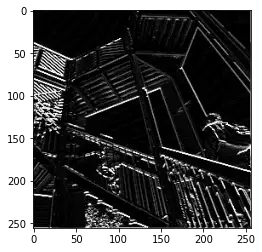 If you look at the axis, the axis is now -- it's 256x256. And if we look at our original image, it was 512x512. This is the original image after the filter.
So you've had a look at how filters can convolve images, providing the basis of convolutional layers, as well as how pooling can reduce the image size while maintaining the features of an image.
In the next part, you'll start implementing convolutions and pooling in code, and you'll see how these can improve the fashion MNIST classifier. After that, you'll take on some more real-world and more challenging images. And you can learn how convolutions can help you to classify them.
Next: Part 4 - Coding with Convolutional Neural Networks

No comments yet