
In this article we're going to look at how to use convolutional neural networks to classify complex features. In previsous part 4 - Coding with Convolutional Neural Networks, you took what you had learned about CNNS. And you saw how to improve the fashion classifier that you had created much earlier on.
So in this part, we'll see if we can apply that to other images like these. 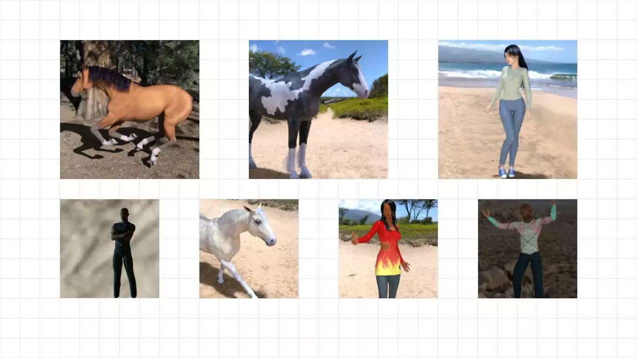 This is a data set of horses and humans with a number of pictures of different horses in different positions, as well as different, very diverse humans also in different poses.
So for example, consider the horse in the top middle. You can only see three of its legs. In the one at the bottom, you can only see two. The men and women are also in different poses. And some have parts of their body obscured. Like the woman with the red dress is actually cut off at the knees.
As you can hopefully see, this is a far more challenging problem than we had with fashion mnist and handwriting digits, where every item was posed similarly. The first thing that we need to do before we start coding our network is to have an easy way to label these images, where we can tell the computer which ones are horses and which ones are humans.
One way to do this that TensorFlow supports to make your life easier is to use sub directories. 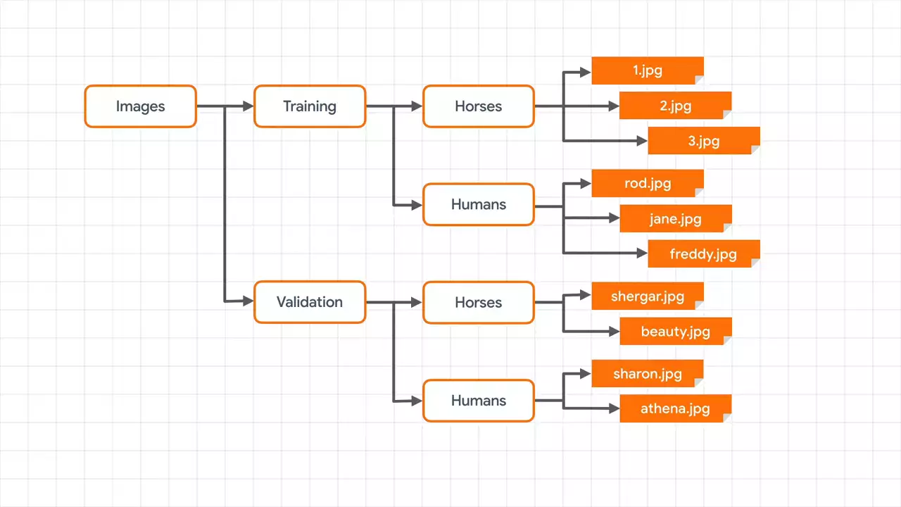 So if I have a master directory of images, and I then subdivide that into training and validation images, and the training directory contains sub directories called horses and humans -- each containing the appropriate images with horses in the horses directory and humans in the humans directory -- and similarly, if I have a validation directory containing horses and humans in sub folders, I now have a fully labeled set of images for training and testing.
With TensorFlow, I can pass these directories to something called a generator. And it will auto label the images based on the directory name.
This labeling is achieved using an image data generator in the Keras libraries. You import it like this.
from tensorflow.keras.preprocessing.image import ImageDataGenerator
You can then use this to do some transforms on the image, such as normalizing them.
# All images will be rescaled by 1./255
train_datagen = ImageDataGenerator(rescale=1/255)

# Flow training images in batches of 128 using train_datagen generator
train_generator = train_datagen.flow_from_directory(
        '/tmp/horse-or-human/',  # This is the source directory for training images
        target_size=(300, 300),  # All images will be resized to 150x150
        batch_size=128,
        # Since we use binary_crossentropy loss, we need binary labels
        class_mode='binary')
This is a very simple normalization where I just divide each channel by 255. There's better ways of doing that. But I'll keep it simple for now. You then create a generator for the images by flowing them out of the directory by calling the flow_from_directory method. You specify the directory that contains the label sub directories.
So for example, in this case, we're training. So this will be the training directory that contains the horses and humans sub directories. It's a common area to use one of those instead. Make sure to use the parent directory.
You need to specify the size of the images that the generator will provide to the model a little later. Remember when, we did the fashion images, they were all 28x28. When using real world images, you aren't guaranteed to have them all the same size. So thus, when flowing them from the directory as well as rescaling, it's a good idea to resize them, too. You can specify the batch size for training. So for example, in this case, they'll be taken from the directory 128 at a time in order to be fed into the neural network.
And finally, there's the class_mode. Keep an eye on this, as it's an easy source of bugs. If you only have two classes like we do here, keep this as binary. If you have more classes, it should be categorical.
For your validation data set, you do exactly the same, except that you create a validation generator and point it at a validation directory.
validation_datagen = ImageDataGenerator(rescale=1/255)

# Flow training images in batches of 128 using train_datagen generator
validation_generator = validation_datagen.flow_from_directory(
        '/tmp/validation-horse-or-human/',  # This is the source directory for training images
        target_size=(300, 300),  # All images will be resized to 150x150
        batch_size=32,
        # Since we use binary_crossentropy loss, we need binary labels
        class_mode='binary')
These two generators now provide the images that your model can use for training and validation. So now it's time to define your model architecture that can use these. And later, we'll see how you can use them when you're fitting your images to your labels.
Here's the code for simple CNN that can classify the horses and humans images.
model = tf.keras.models.Sequential([
    tf.keras.layers.Conv2D(16, (3,3), activation='relu',
                           input_shape=(300, 300, 3)),
    tf.keras.layers.MaxPooling2D(2, 2),
    tf.keras.layers.Conv2D(32, (3,3), activation='relu'),
    tf.keras.layers.MaxPooling2D(2,2),
    tf.keras.layers.Conv2D(64, (3,3), activation='relu'),
    tf.keras.layers.MaxPooling2D(2,2),
    tf.keras.layers.Flatten(),
    tf.keras.layers.Dense(512, activation='relu'),
    tf.keras.layers.Dense(1, activation='sigmoid')
])
This should look a little familiar by now. First is a few stacked convolutional layers, where every convolutional layer is followed by a max pooling one, as we saw on the previous part. The number of convolutions in each layer is purely arbitrary. You can experiment to get the best results. I've done it here by increasing the number of filters as the image size decreases. Remember that the pooling layer is quarter the size of your image. So at the smaller images, I'm trying more filters. But you're free to experiment.
Remember the input shape, though. That's super important. Here, we're telling the initial layer to expect to be fed data in a 300x300x3 format. So each image is 300x300 pixels. And there are three bytes per pixel. This needs to match the size that you specified in the generator a little earlier.
Finally is your output layer. The number of neurons should match the number of classes that you have. There is one exception. With a binary classifier, you can get away with only one neuron and a sigmoid activation function. And this pushes the value towards 0 for one class and towards 1 for the other class.
If we look at our model architecture, we'll see something like this.
Model: "sequential"
_________________________________________________________________
Layer (type)                 Output Shape              Param #
=================================================================
conv2d (Conv2D)              (None, 298, 298, 16)      448
_________________________________________________________________
max_pooling2d (MaxPooling2D) (None, 149, 149, 16)      0
_________________________________________________________________
conv2d_1 (Conv2D)            (None, 147, 147, 32)      4640
_________________________________________________________________
max_pooling2d_1 (MaxPooling2 (None, 73, 73, 32)        0
_________________________________________________________________
conv2d_2 (Conv2D)            (None, 71, 71, 64)        18496
_________________________________________________________________
max_pooling2d_2 (MaxPooling2 (None, 35, 35, 64)        0
_________________________________________________________________
flatten (Flatten)            (None, 78400)             0
_________________________________________________________________
dense (Dense)                (None, 512)               40141312
_________________________________________________________________
dense_1 (Dense)              (None, 1)                 513
=================================================================
Total params: 40,165,409
Trainable params: 40,165,409
Non-trainable params: 0
And the journey of the image through the layers is apparent. It starts 300x300, loses a pixel border to become to 298x298, gets halved in each dimension by the pooling to become 149x149, and it loses another pixel border, et cetera, et cetera. Overall, this network will need to learn about 40 million parameters. So training might take a little while.
When you compile your model, you specify a loss function and an optimizer.
from tensorflow.keras.optimizers import RMSprop

model.compile(loss='binary_crossentropy',
              optimizer=RMSprop(lr=0.001),
              metrics=['accuracy'])
In this case, we're going to use a loss function called binary_crossentropy. And this is a common one when there's a binary classification. We'll also use an optimizer called RMSprop, which is able to accept parameters for something called the learning rate. Start with 0.001. And you can tweak it as you go. And we'll capture the accuracy matrix while we're training.
The learning rate parameter defines how the mathematical functions in the transformer can learn using something called gradient descent. It's a little bit beyond this tutorial to go into that in detail.
Now it's time to do the training.
history = model.fit(
      train_generator,
      validation_data = validation_generator,
      epochs=15,
      verbose=2)
And if you're familiar with model.fit, which we saw previously, where we specified the data and the labels when using a generator, all you have to do is specify the generator. And it will infer the labels from the provided sub directories. And you can see that here. My training data. And that has the images and the labels that are provided by the training generator. I'll just train it for a short time, 15 epochs. And you'll see how well this model can perform. The validation data will come from the validation generator. And in the same way as the training, it will get both the images and the labels. The verbose parameter just tells TensorFlow how much detail to report per epoch.
If you remember back when we specified the training generator and we defined batch sizes to flow the images from the directory. You can also specify the batches for training. And you'll find that training will be drastically faster. It takes a bit of experimentation to get the right combination. But when I didn't use any, using Colab, even with a GPU, it was taking many minutes per epoch. However, if I specify the number of steps to use when training, it massively increases performance so that each epoch was taking less than 10 seconds. So watch out for this while you're training.
Here's the code with the step set.
history = model.fit(
      train_generator,
      validation_data = validation_generator,
      epochs=15,
      steps_per_epoch=8,
      validation_steps=8,
      verbose=1)
The rule of thumb here is to consider the amount of items in the data set and then divide it by the batch size. If you remember earlier, we had 128 batch size. And there's a little over 1,024 items in the data set. So I chose a step size of eight.
After 15 epochs, this model should reach close to 100% accuracy on the training set and about 85% on the validation set. This is called overfitting. And it's a common error in neural networks that can lead you to a false sense of security. What has happened is that the network got to be really, really good, almost perfect at classifying data that it has already seen. And that's the training data. But it's not quite as good at understanding data that it hadn't previously seen, such as the stuff in the validation data set.
It's a little bit like if the only shoes you had ever seen in your life were hiking boots. Then, you may not recognize a high heel as a shoe. You've overfit yourself into thinking that all shoes look like hiking boots. There are techniques to avoid this in neural networks. And we'll look at some of them soon. But before that, let's just explore how to use the network that you've just created to classify images.
Here's the code to upload an image to Colab and have it use the model to predict the contents of the image.
import numpy as np
from google.colab import files
from keras.preprocessing import image

uploaded = files.upload()

for fn in uploaded.keys():

  # predicting images
  path = '/content/' + fn
  img = image.load_img(path, target_size=(300, 300))
  x = image.img_to_array(img)
  x = x / 255
  x = np.expand_dims(x, axis=0)
  images = np.vstack([x])
  classes = model.predict(images, batch_size=10)
  print(classes[0])
  if classes[0]>0.5:
    print(fn + " is a human")
  else:
    print(fn + " is a horse")
This works in Colab only. And you import the files library to use it. And to get a list of uploaded files by calling files.upload. Then, for each file that's uploaded, you have to convert it to be 300x300, turn it into an array, and call expand_dims to ensure that it's a three-dimensional array with the third element being the color depth that we saw when we were defining the model.
Once you have your image or images in a list, you can then call model.predict to get the results back. If the value is greater than 0.5, it's a human. Otherwise, it's a horse.
Next: Part 6 - Convolutional cats and dogs

No comments yet